Missingness in Pew Research Center’s Latin American Religion Dataset
8 minutes
Introduction #
Latin America is a large region with many different faith traditions. Latin American countries were without exception historically tied to Catholicism due to the region’s colonization by the Spanish and other European countries. The Pew Research Survey on Religion in Latin America shows the rapid growth of Protestant populations throughout Latin America. Generational cultural differences are often key to one’s political and social positions. The Survey on Religion in Latin America also showed that in some countries, there are more men than women who say that homosexuality is morally wrong. These dynamics are important to consider when looking at studies on the subject of gay marriage. This paper aims to explore to what extent religious affiliation, gender, and age correlate with support for gay marriage.
Data #
In this paper, we will be looking at data from the Pew Research Center’s Survey on Religion in Latin America. The survey was conducted from October 2013 to February 2014 through face-interviews at the respondent’s places of residence in Costa Rica, El Salvador, Honduras, Mexico, Nicaragua, Panama, Argentina, Bolivia, Brazil, Chile, Colombia, the Dominican Republic, Ecuador, Paraguay, Peru, Uruguay, Venezuela, and Puerto Rico. The data dictionary mentions that all samples were based on multi-stage cluster designs. The survey included questions about religious and social views. The dataset includes 323, but the four we will be using in our analysis are listed below.
- marriageSupport: Answer to the question “Do you strongly favor, favor, oppose, or strongly oppose allowing gays and lesbians to marry legally?”, turned into a binary outcome.
- religionQ : Answer to the question “What is your present religion?” Responses include Roman Catholic, Evangelical/Protestant, Other Religion, and Unaffiliated
- age: The age of the respondent on their last birthday up to 97 years
- gender: gender recorded by the observation of the interviewer
Methods #
This project will explore different missing data methods, such as Multiple Imputation Chained Equations (MICE), mean imputation, and complete case analysis.
Complete case analysis is the most convenient method available to deal with missing data. It entails removing any observation with a missing value and proceeding with the analysis. One of the drawbacks of this method is that we might be ignoring a large amount of data, which might introduce bias to our results.
The next method we’ll be using is predictive mean matching. For each missing entry, the method forms a set of candidate donors and randomly selects one to impute according to a specified imputation model. The advantages of this method are that all imputed values are plausible and can be applied to any type of variable.
The last method we’ll be using is Multiple Imputation Using Chained Equations (MICE). We will be using 20 imputed datasets with 20 iterations each for robustness. The advantage of this method are that we are able to obtain unbiased estimates for the target estimand and variance.
We will be fitting a logistic regression model to estimate whether a person supports gay marriage based on age, religous affiliation, and gender.
Results #
Missingness #
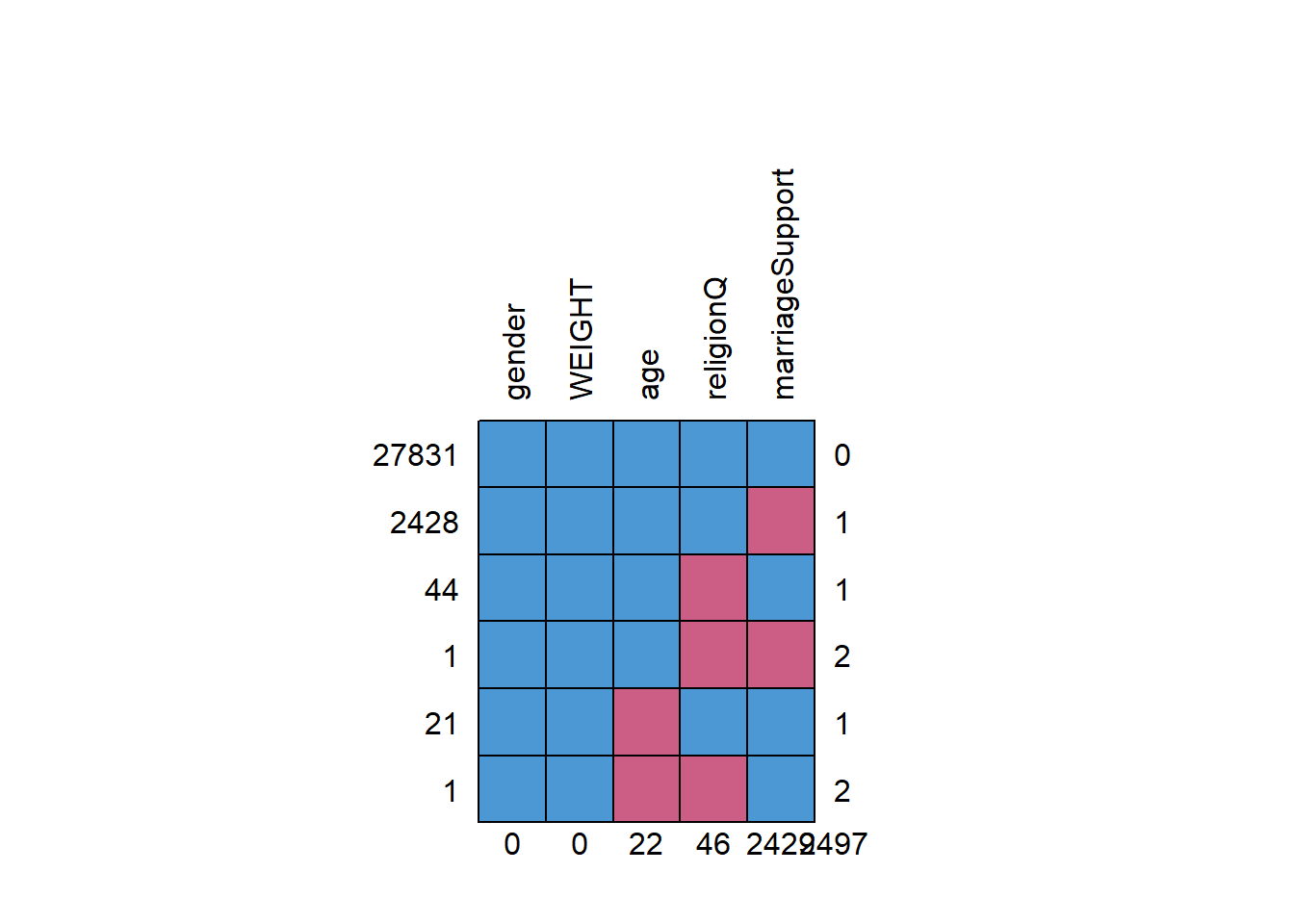
In the Pew Research Center’s Dataset, missing values are coded as 98 and 99. After cleaning up the data, we observed the missingness pattern below.
##       gender WEIGHT age religionQ marriageSupport
## 27831      1      1   1         1               1    0
## 2428       1      1   1         1               0    1
## 44         1      1   1         0               1    1
## 1          1      1   1         0               0    2
## 21         1      1   0         1               1    1
## 1          1      1   0         0               1    2
##            0      0  22        46            2429 2497
## marriageSupport       religionQ          gender             age          WEIGHT
##    0.0800962870    0.0015168502    0.0000000000    0.0007254501    0.0000000000
We can see that the marriageSupport column has 2429 missing values, which is about 8% of the observations. There were 22 observations with age missing, and 46 with religious affiliation missing. Most of the missing values are non-monotone and not connected. There are only 2 observations with two missing values.
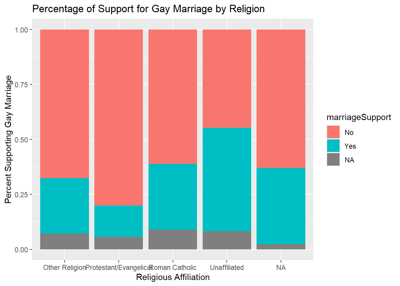
After inspecting the plot, we can see that a majority of people with a religious affiliation are opposed to gay marriage. There seems to be an equal amount of unaffiliated respondents that support and oppose gay marriage. There also seems to be roughly equal percent of missingness in marriageSupport across different religious affiliations.
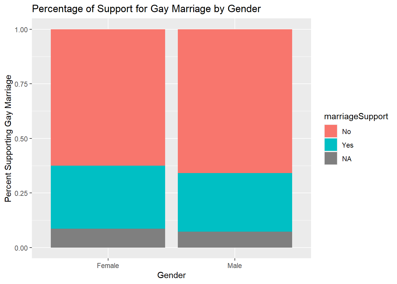
The percentage of respondents who oppose and support gay marriage seems to be roughly equal for males and females. There also seems to be a roughly equal percentage of respondents who did not answer the question for males and females.
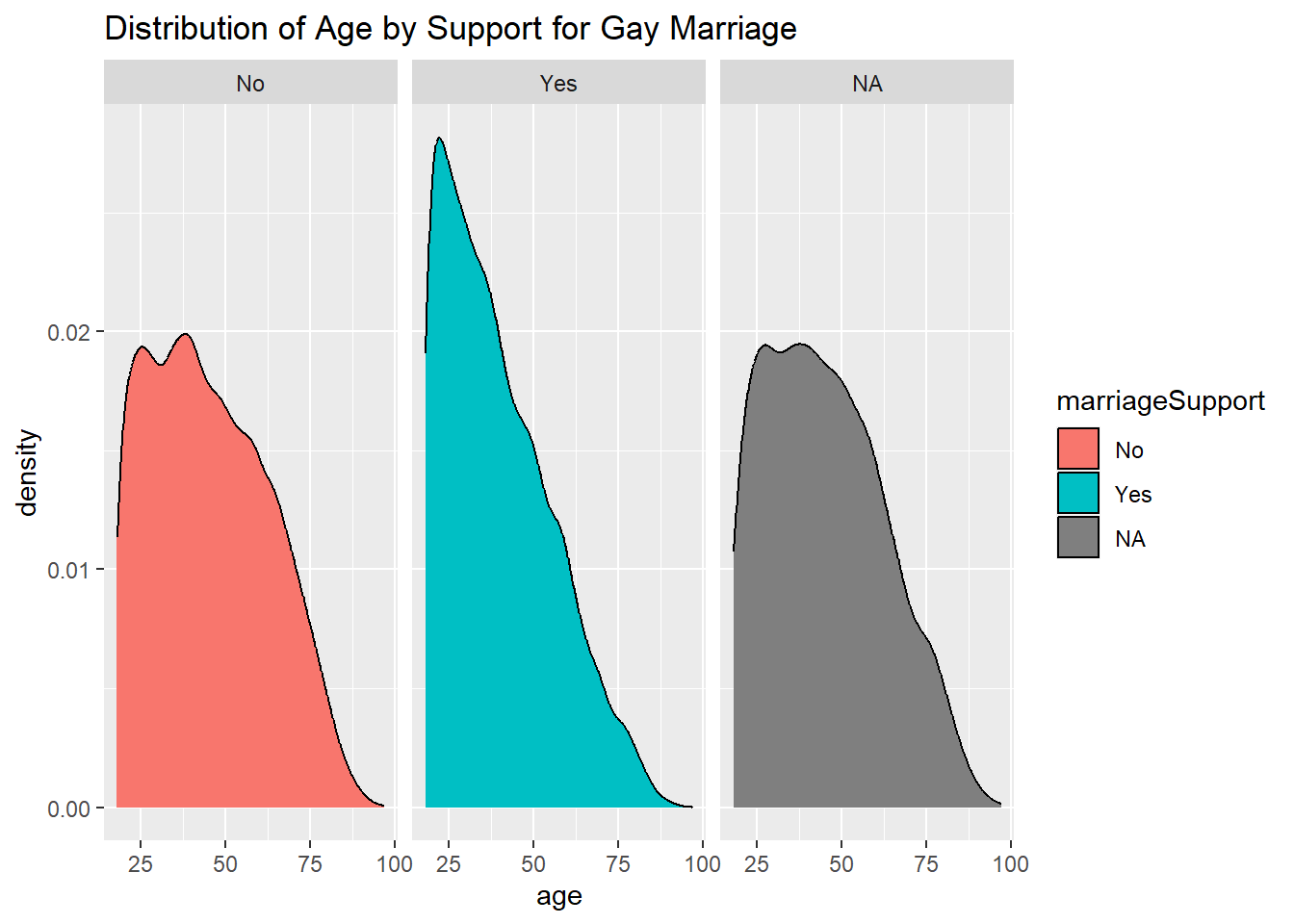
The distribution of age for respondents who oppose gay marriage and those who did not respond are similar. The distribution of respondents who favor gay marriage is greatly concentrated around the younger demographic.
Application #
Next, we apply logistic regression to complete datasets generated by the missing data methods discussed earlier.
| 2.5 % | 97.5 % | ||
|---|---|---|---|
| (Intercept) | 1.1011609 | 0.9329282 | 1.2967976 |
| age | 0.9778216 | 0.9762123 | 0.9794254 |
| religionQProtestant/Evangelical | 0.4509692 | 0.3831010 | 0.5320840 |
| religionQRoman Catholic | 1.3609587 | 1.1697589 | 1.5879732 |
| religionQUnaffiliated | 2.4309172 | 2.0560642 | 2.8809012 |
| genderMale | 0.8053418 | 0.7639813 | 0.8488939 |
For the complete case analysis, a total of 2,495 out of 30,326 observations were removed.
| 2.5 % | 97.5 % | ||
|---|---|---|---|
| (Intercept) | 1.0579570 | 0.9014491 | 1.2388872 |
| age | 0.9781089 | 0.9765742 | 0.9796386 |
| religionQProtestant/Evangelical | 0.4664757 | 0.3983385 | 0.5474894 |
| religionQRoman Catholic | 1.4201554 | 1.2267277 | 1.6486770 |
| religionQUnaffiliated | 2.5539623 | 2.1723950 | 3.0094529 |
| genderMale | 0.7980469 | 0.7587354 | 0.8393491 |
Our coefficients for logistic regression using predictive mean matching are similar.
| term | estimate | 2.5 % | 97.5 % |
|---|---|---|---|
| (Intercept) | 1.0356372 | 0.8768544 | 1.2231728 |
| age | 0.9782189 | 0.9766100 | 0.9798305 |
| religionQProtestant/Evangelical | 0.4506852 | 0.3819931 | 0.5317298 |
| religionQRoman Catholic | 1.3521861 | 1.1582396 | 1.5786088 |
| religionQUnaffiliated | 2.6070107 | 2.1980815 | 3.0920167 |
| genderMale | 0.8220291 | 0.7792023 | 0.8672098 |
There doesn’t seem to be much difference in the results superficially. All coefficients, except for the intercept, have significant associations with whether or not a respondent supports the legalization of gay marriage.
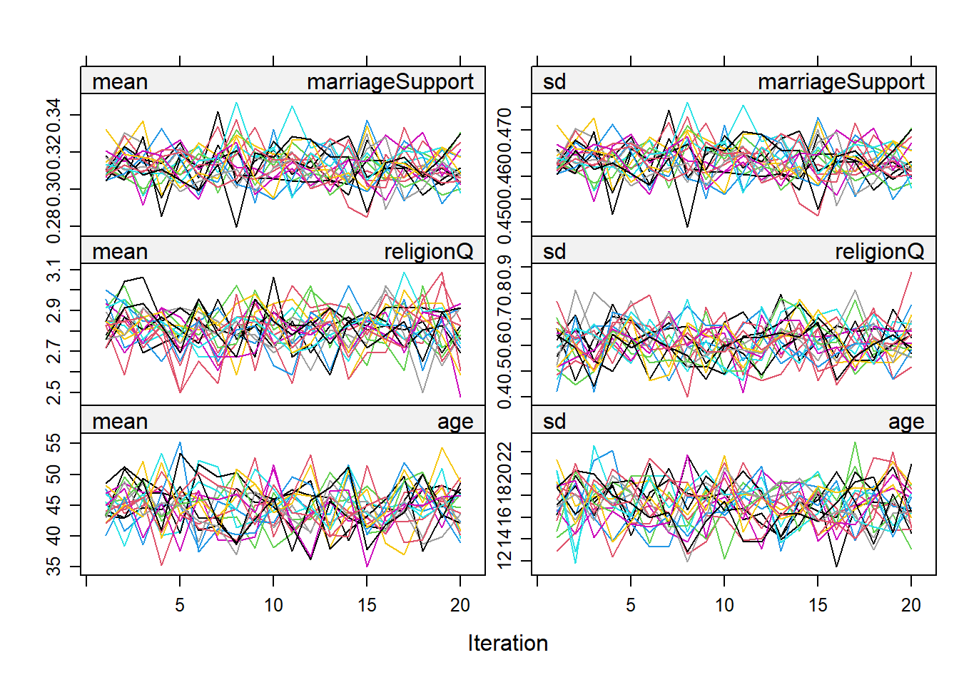
The convergence plot seems to show that the streams for mean and variance for all three variables intermingle and have no pattern, so we can say that they converge.
Dicussion #
In conclusion, all three of our logistic regression models are pretty similar. All of the explanatory variables were shown to be significant. The logistic regression model built with MICE suggests there is, on average, about a 2% decrease in the odds a respondent supports gay marriage for each unit increase in age. There is about a 65% decrease, on average, in the odds a respondent supports gay marriage if the respondent identifies as Protestant/Evangelical. There is about a 35% increase, on average, in the odds a respondent supports gay marriage if the respondent identifies as Roman Catholic. There is about a 160% increase, on average, in the odds a respondent supports gay marriage if the respondent identifies as Unaffiliated. There is about a 18% decrease, on average, in the odds a respondent supports gay marriage if the respondent was identified as male.
Our results suggests that religious affiliation, age, and gender of someone in Latin America is associated with whether they support or oppose the legalization of gay and lesbian marriage. The Pew Research Dataset on Religion in Latin America presents many questions to explore. Are there differences in doctrine between Protestants and Catholics that explains the difference in support for the outcome? A next step would be to see what denominations of people within the Protestant/Evangelical have greater opposition to gay marriage.
Appendix #
Reading and Cleaning Data #
religion <- read_sav("./ReligionLatinAmerica/Religion.sav")

religion_1 <- religion %>%
  select(Q15, QCURRELrec, Q73, Q74, WEIGHT) %>%
  mutate(marriageSupport = ifelse(Q15 >= 98, NA_real_, ifelse(Q15 <= 2, 1, 0)),
         religionQ = ifelse(QCURRELrec >= 98, NA_real_,
                            recode(QCURRELrec,"Roman Catholic",
                                   "Protestant/Evangelical", "Other Religion",
                                   "Unaffiliated")),
         gender = ifelse(Q73 == 1, "Male", "Female"),
         age = ifelse(Q74 >= 98, NA_real_, Q74),
         religionQ = as.factor(religionQ),
         gender = as.factor(gender)) %>%
  select(marriageSupport, religionQ, gender, age)
Exploratory Plots #
ggplot(religion_1, aes(x = marriageSupport, fill = marriageSupport)) +
  geom_bar() +
  facet_wrap(~religionQ, nrow = 1) +
  labs(title = "Count of Support for Gay Marriage by Religion",
       x = "Support for Gay Marriage")+
  theme(legend.position = "none")

ggplot(religion_1, aes(x = marriageSupport, fill = marriageSupport)) +
  geom_bar() +
  facet_wrap(~gender, nrow = 1) +
  labs(title = "Count of Support for Gay Marriage by Gender",
       x = "Support for Gay Marriage") +
  theme(legend.position = "none")

ggplot(religion_1, aes(x = age , fill = marriageSupport)) +
  geom_density() +
  facet_wrap(~marriageSupport) +
  labs(title = "Distribution of Age by Support for Gay Marriage") +
  theme(legend.position = "none")
Missingness Plot #
md.pattern(religion_1, rotate.names = TRUE)
Percent missing #
colSums(is.na(religion_1)) / nrow(religion_1)
Complete Case Analysis #
religion_omit <- religion_1 %>%
  na.omit()

religion_omit_model <- with(religion_omit,
                            glm(marriageSupport ~ age + religionQ + gender,
                                family = binomial(link="logit"),
                                weights = religion_omit$WEIGHT))

summary(religion_omit_model)

tbl_complt <- cbind(
  exp(summary(religion_omit_model, confint = TRUE)$coefficients[,1]),
  exp(confint(religion_omit_model)))

tbl_complt %>%
  kable(caption = "Logistic Regression Complete Case")
Predictive Mean Matching #
religion_pmm <- mice(religion_1, m = 1, maxit = 1, method = "pmm",
                     printFlag = FALSE) %>%
  complete()

religion_pmm_model <- with(religion_pmm,
                           glm(marriageSupport ~ age + religionQ + gender,
                               family = binomial(link="logit"),
                               weights = religion_pmm$WEIGHT))

summary(religion_pmm_model)

tbl_pmm <- cbind(
  exp(summary(religion_pmm_model, confint = TRUE)$coefficients[,1]),
  exp(confint(religion_pmm_model)))

tbl_pmm %>%
  kable(caption = "Logistic Regression with Predictive Mean Matching")
Multiple Imputation #
imp <- mice(religion_1, m = 20, maxit = 20,method = "pmm", printFlag = FALSE)
MICE plots #
plot(imp)
Pooling MICE #
# Applying logistic regression to imputed dataset
religion_imp_model <- with(imp, glm(marriageSupport ~ age + religionQ + gender,
                                    family = binomial(link = 'logit'),
                                    weights = imp$WEIGHT))

# Pooling results
pooled_religion <- pool(religion_imp_model)

summary(pooled_religion)

# Confidence interval for logistic regression coefficients
summary(pooled_religion, conf.int = TRUE, exp= TRUE)[,c("term", "estimate",
                                                        "2.5 %", "97.5 %")] %>%
  kable(caption = "Logistic Regression with MICE")